中级绘图
1、散点图
1 2 3 4 5 6 7
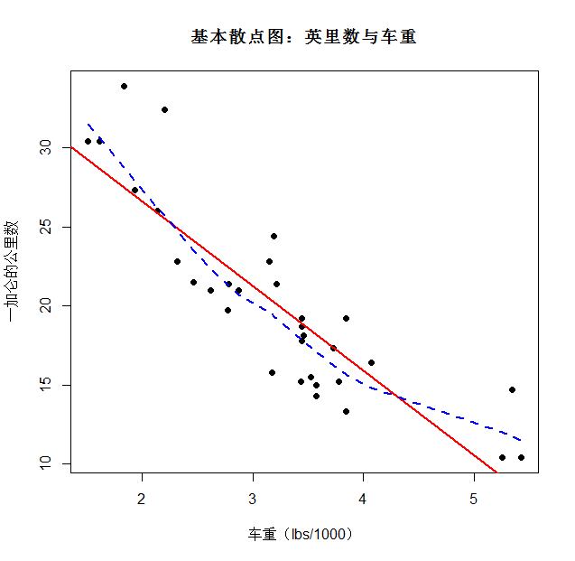
| attach(mtcars) plot(wt,mpg,main="基本散点图:英里数与车重",xlab = "车重(lbs/1000)",ylab="一加仑的公里数",pch=19) abline(lm(mpg~wt),col="red",lwd=2,lty=1) lines(lowess(wt,mpg),col="blue",lwd=2,lty=2)
|
1 2
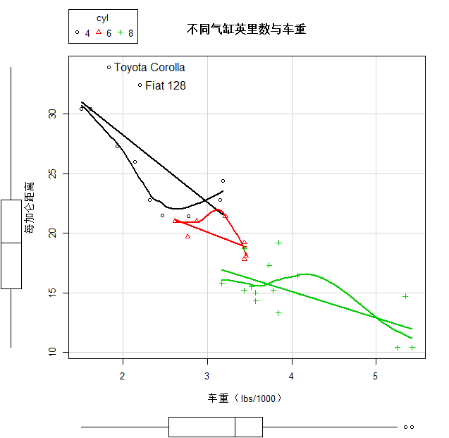
| library(car) scatterplot(mpg~wt|cyl,data=mtcars,lwd=2,main="不同气缸英里数与车重",xlab="车重(lbs/1000)",ylab="每加仑距离",legend.plot=TRUE,id.method="identify",labels=row.names(mtcars),boxplots="xy")
|
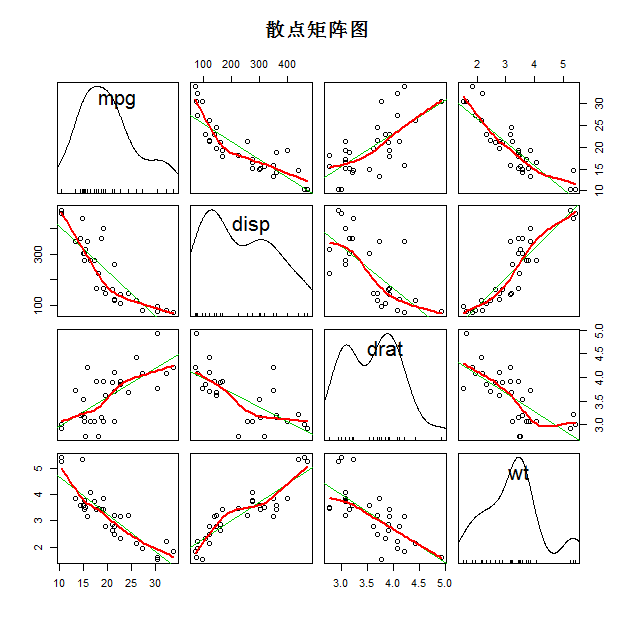
1.1、散点矩阵图
1 2 3 4
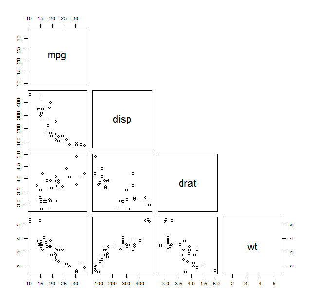
| plot(~mpg+disp+drat+wt,data=mtcars) pairs(~mpg+disp+drat+wt,data=mtcars,upper.panel = NULL)
|

1 2 3 4
| library(car) scatterplotMatrix(~mpg+disp+drat+wt,data=mtcars,spread=FALSE,lty.smooth=2,main="散点矩阵图")
|
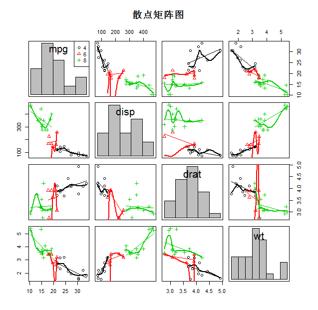
1 2
| scatterplotMatrix(~mpg+disp+drat+wt|cyl,data=mtcars,by.groups = TRUE,diagonal="histogram",main="散点矩阵图")
|
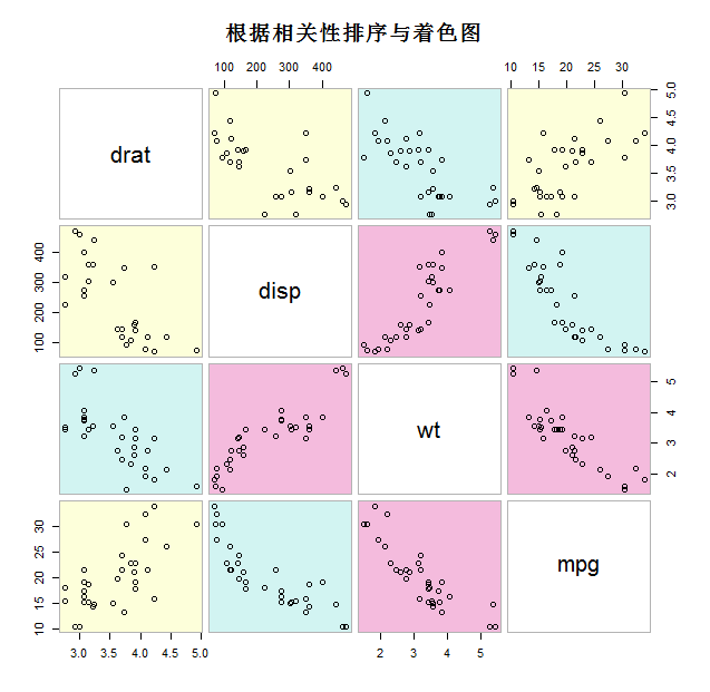
1 2 3 4 5 6 7 8 9 10
| library(gclus) mydata<-mtcars[c(1,3,5,6)] mydata.corr<-abs(cor(mydata)) mycolors<-dmat.color(mydata.corr) myorder<-order.single(mydata.corr) cpairs(mydata,myorder,panel.colors = mycolors,gap=.5,main="根据相关性排序与着色图")
|
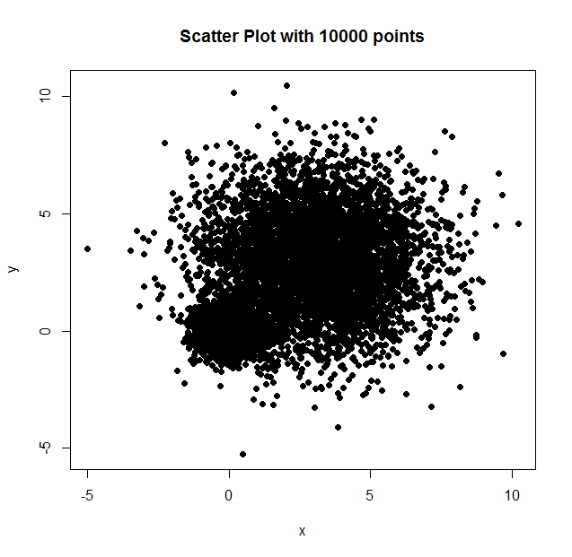
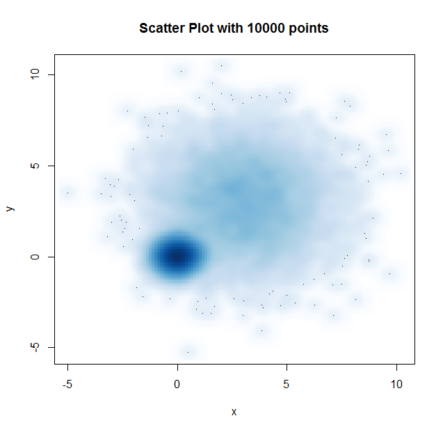
1.2、高密度散点图
1 2 3 4 5 6 7 8 9
| set.seed(1234) n<-10000 c1<-matrix(rnorm(n,mean = 0,sd=0.5),ncol=2) c2<-matrix(rnorm(n,mean = 3,sd=2),ncol=2) mydata<-rbind(c1,c2) mydata<-as.data.frame(mydata) names(mydata)<-c("x","y") with(mydata,plot(x,y,pch=19,main="Scatter Plot with 10000 points"))
|
1
| with(mydata,smoothScatter(x,y,main="Scatter Plot with 10000 points"))
|
1 2 3 4 5
| library(hexbin) with(mydata,{ bin<-hexbin(x,y,xbins=50) plot(bin,main="六边形散点图") })
|

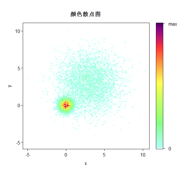
1 2
| library(IDPmisc) with(mydata,iplot(x,y,main="颜色散点图"))
|
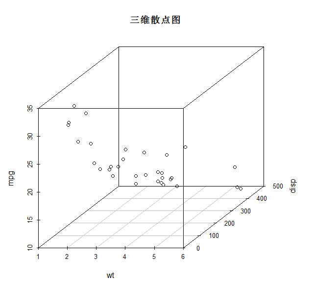
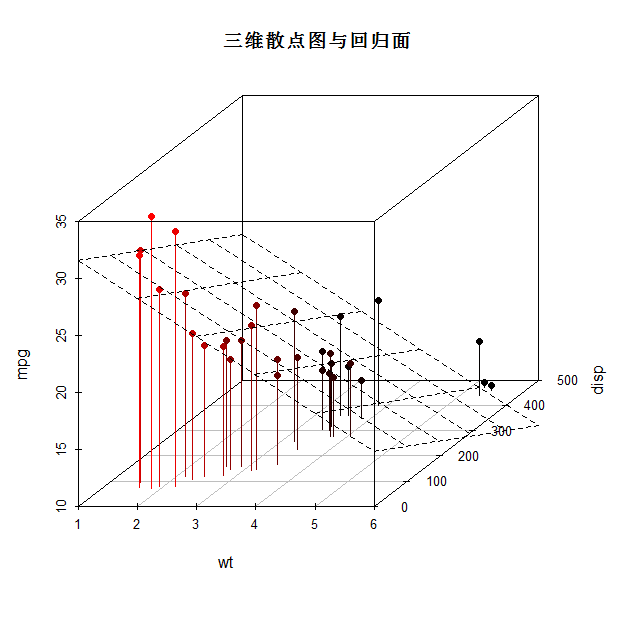
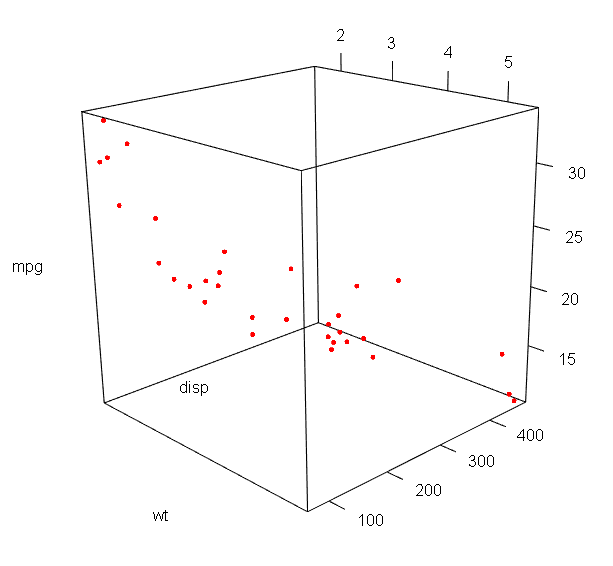
1.3、三维散点图
1 2 3
| library(scatterplot3d) attach(mtcars) scatterplot3d(wt,disp,mpg,main="三维散点图")
|
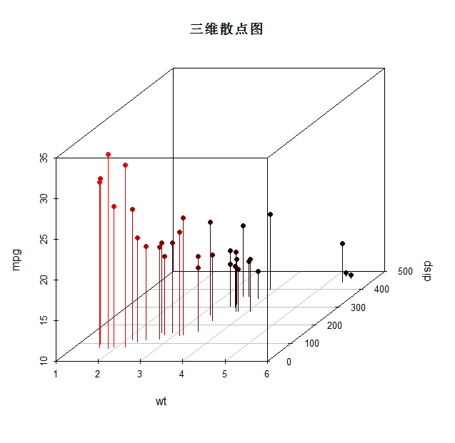
1 2
| scatterplot3d(wt,disp,mpg,pch=16,highlight.3d=TRUE,type="h",main="三维散点图")
|
1 2 3 4
| s3d<-scatterplot3d(wt,disp,mpg,pch=16,highlight.3d=TRUE,type="h",main="三维散点图与回归面") fit<-lm(mpg~wt+disp) s3d$plane3d(fit)
|
1 2 3 4
| library(rgl) attach(mtcars) plot3d(wt,disp,mpg,col="red",size=5)
|
1 2 3
| library(Rcmdr) scatter3d(wt,disp,mpg)
|

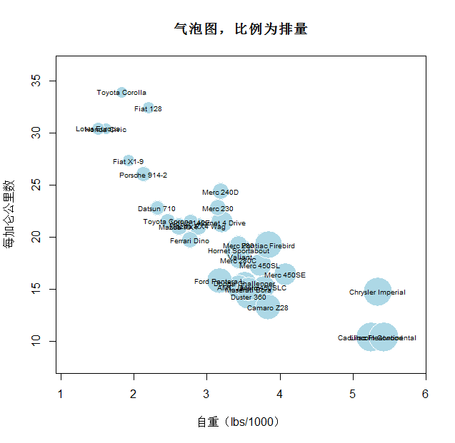
1.4、气泡图
1 2 3 4 5
| r<-sqrt(disp/pi) symbols(wt,mpg,circle=r,inches = 0.30,fg="white",bg="lightblue",main="气泡图,比例为排量", ylab="每加仑公里数",xlab="自重(lbs/1000)") text(wt,mpg,rownames(mtcars),cex=0.6)
|
2、折线图
1 2 3 4 5 6 7 8 9 10 11 12 13 14 15 16 17 18 19 20 21 22 23 24 25 26 27 28
| Orange$Tree<-as.numeric(Orange$Tree) ntrees<-max(Orange$Tree) xrange<-range(Orange$age) yrange<-range(Orange$circumference) plot(xrange,yrange,type="n", xlab="树龄/天",ylab="直径/mm") colors<-rainbow(ntrees) linetype<-c(1:ntrees) plotchar<-seq(18,18+ntrees,1) for(i in 1:ntrees){ tree<-subset(Orange,Tree==i) lines(tree$age,tree$circumference, type="b",lwd=2, lty=linetype[i], col=colors[i], pch=plotchar[i]) } title("树图","折线示例") legend(xrange[1],yrange[2], 1:ntrees,cex=0.8,col=colors,pch=plotchar,lty=linetype,title="Tree")
|

3、相关图
1 2 3 4 5 6 7 8 9 10 11 12 13 14
| library(corrgram) corrgram(mtcars,order=TRUE,lower.panel = panel.shade,upper.panel = panel.pie,text.panel = panel.txt, main="相关系数图")
|

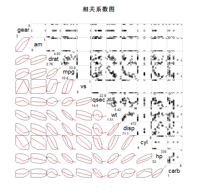
1 2 3 4 5 6
| corrgram(mtcars,order=TRUE, lower.panel = panel.ellipse, upper.panel = panel.pts, text.panel = panel.txt, diag.panel = panel.minmax, main="相关系数图")
|
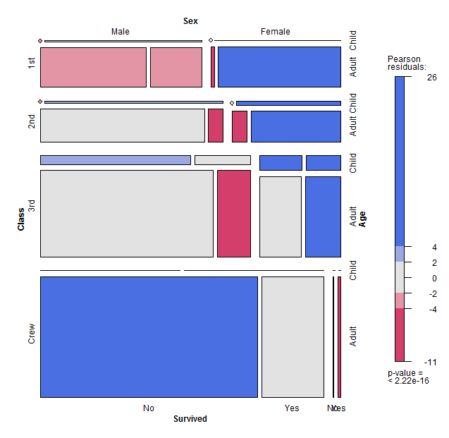
4、马赛克图
1 2 3 4 5 6 7 8 9
| library(vcd) ftable(Titanic) mosaic(Titanic,shade = TRUE,legend=TRUE)
|