文章目录
  1. 广义线性模型
    1. 1、广义线性模型和glm函数、logistics回归
    2. 2、logistics的过度离势
    3. 3、logistics的扩展
    4. 4、泊松回归
    5. 5、泊松回归的过度离势

广义线性模型

1、广义线性模型和glm函数、logistics回归

1
2
3
4
5
6
7
8
9
10
11
12
13
14
15
16
17
18
19
20
21
22
23
24
25
26
27
28
29
30
31
32
33
34
35
36
37
38
39
40
41
42
43
44
45
46
47
48
49
50
51
52
53
54
55
56
57
58
59
60
61
62
63
64
65
66
67
68
69
70
71
72
73
74
75
76
77
78
79
80
81
82
83
84
85
86
87
88
89
90
91
92
93
94
95
96
97
98
99
100
101
102
103
104
105
106
107
108
109
110
111
112
113
114
115
116
117
118
119
120
121
122
123
124
125
126
127
128
129
130
131
132
133
134
135
136
137
138
139
140
141
142
143
144
145
146
147
148
149
150
151
152
153
154
155
156
157
158
159
160
161
162
163
164
> #使用glm函数进行处理,可以分析多种分布,二分,多值,数值等,此处不限制因变量Y为服从正态分布
> #Logistic回归
>
> library(AER)
> data("Affairs",package = "AER")
> summary(Affairs)
affairs gender age yearsmarried children religiousness
Min. : 0.000 female:315 Min. :17.50 Min. : 0.125 no :171 Min. :1.000
1st Qu.: 0.000 male :286 1st Qu.:27.00 1st Qu.: 4.000 yes:430 1st Qu.:2.000
Median : 0.000 Median :32.00 Median : 7.000 Median :3.000
Mean : 1.456 Mean :32.49 Mean : 8.178 Mean :3.116
3rd Qu.: 0.000 3rd Qu.:37.00 3rd Qu.:15.000 3rd Qu.:4.000
Max. :12.000 Max. :57.00 Max. :15.000 Max. :5.000
education occupation rating
Min. : 9.00 Min. :1.000 Min. :1.000
1st Qu.:14.00 1st Qu.:3.000 1st Qu.:3.000
Median :16.00 Median :5.000 Median :4.000
Mean :16.17 Mean :4.195 Mean :3.932
3rd Qu.:18.00 3rd Qu.:6.000 3rd Qu.:5.000
Max. :20.00 Max. :7.000 Max. :5.000
> Affairs$ynAffair[Affairs$affairs > 0 ] <- 1
> Affairs$ynAffair[Affairs$affairs == 0 ] <- 0
>
> Affairs$ynAffair <- factor(Affairs$ynAffair, levels = c(0,1), labels = c("No", "Yes"))
>
> table (Affairs$ynAffair)
No Yes
451 150
>
> fit.full <- glm(ynAffair ~ gender + age + yearsmarried + children + religiousness + education + occupation + rating, data=Affairs,family = binomial())
> summary(fit.full)
Call:
glm(formula = ynAffair ~ gender + age + yearsmarried + children +
religiousness + education + occupation + rating, family = binomial(),
data = Affairs)
Deviance Residuals:
Min 1Q Median 3Q Max
-1.5713 -0.7499 -0.5690 -0.2539 2.5191
Coefficients:
Estimate Std. Error z value Pr(>|z|)
(Intercept) 1.37726 0.88776 1.551 0.120807
gendermale 0.28029 0.23909 1.172 0.241083
age -0.04426 0.01825 -2.425 0.015301 *
yearsmarried 0.09477 0.03221 2.942 0.003262 **
childrenyes 0.39767 0.29151 1.364 0.172508
religiousness -0.32472 0.08975 -3.618 0.000297 ***
education 0.02105 0.05051 0.417 0.676851
occupation 0.03092 0.07178 0.431 0.666630
rating -0.46845 0.09091 -5.153 2.56e-07 ***
---
Signif. codes: 0 ‘***’ 0.001 ‘**’ 0.01 ‘*’ 0.05 ‘.’ 0.1 ‘ ’ 1
(Dispersion parameter for binomial family taken to be 1)
Null deviance: 675.38 on 600 degrees of freedom
Residual deviance: 609.51 on 592 degrees of freedom
AIC: 627.51
Number of Fisher Scoring iterations: 4
>
> #去除不显著的因素后再次进行建模
> fit.some <- glm(ynAffair ~ age + yearsmarried + religiousness + rating, data=Affairs,family = binomial())
> summary(fit.some)
Call:
glm(formula = ynAffair ~ age + yearsmarried + religiousness +
rating, family = binomial(), data = Affairs)
Deviance Residuals:
Min 1Q Median 3Q Max
-1.6278 -0.7550 -0.5701 -0.2624 2.3998
Coefficients:
Estimate Std. Error z value Pr(>|z|)
(Intercept) 1.93083 0.61032 3.164 0.001558 **
age -0.03527 0.01736 -2.032 0.042127 *
yearsmarried 0.10062 0.02921 3.445 0.000571 ***
religiousness -0.32902 0.08945 -3.678 0.000235 ***
rating -0.46136 0.08884 -5.193 2.06e-07 ***
---
Signif. codes: 0 ‘***’ 0.001 ‘**’ 0.01 ‘*’ 0.05 ‘.’ 0.1 ‘ ’ 1
(Dispersion parameter for binomial family taken to be 1)
Null deviance: 675.38 on 600 degrees of freedom
Residual deviance: 615.36 on 596 degrees of freedom
AIC: 625.36
Number of Fisher Scoring iterations: 4
>
> #新模型的每个回归系数都非常显著(p<0.05)。由于两模型嵌套(fit.some是fit.full
> #的一个子集),你可以使用anova()函数对它们进行比较,对于广义线性回归,可用卡方检验。
>
> anova(fit.some, fit.full, test = "Chisq")
Analysis of Deviance Table
Model 1: ynAffair ~ age + yearsmarried + religiousness + rating
Model 2: ynAffair ~ gender + age + yearsmarried + children + religiousness +
education + occupation + rating
Resid. Df Resid. Dev Df Deviance Pr(>Chi)
1 596 615.36
2 592 609.51 4 5.8474 0.2108
>
> #卡方值不显著,得知两种模型的解释度是一样的
>
> #回归系数
> coef(fit.some)
(Intercept) age yearsmarried religiousness rating
1.93083017 -0.03527112 0.10062274 -0.32902386 -0.46136144
> #在Logistic回归中,响应变量是Y=1的对数优势比(log)。回归系数含义是当其他预测变量不
> #变时,一单位预测变量的变化可引起的响应变量对数优势比的变化。
>
> #由于对数优势比解释性差,你可对结果进行指数化:
> exp(coef(fit.some))
(Intercept) age yearsmarried religiousness rating
6.8952321 0.9653437 1.1058594 0.7196258 0.6304248
>
> #可以看到婚龄增加一年,婚外情的优势比将乘以1.106(保持年龄、宗教信仰和婚姻评定不
> #变);相反,年龄增加一岁,婚外情的的优势比则乘以0.965。因此,随着婚龄的增加和年龄、宗
> #教信仰与婚姻评分的降低,婚外情优势比将上升。因为预测变量不能等于0,截距项在此处没有
> #什么特定含义。
>
> #还可使用confint()函数获取系数的置信区间。例如, exp(confint(fit.reduced))
> #可在优势比尺度上得到系数95%的置信区间。
> exp(confint(fit.some))
Waiting for profiling to be done...
2.5 % 97.5 %
(Intercept) 2.1255764 23.3506030
age 0.9323342 0.9981470
yearsmarried 1.0448584 1.1718250
religiousness 0.6026782 0.8562807
rating 0.5286586 0.7493370
>
> #以概率的方式思考比使用优势比更直观。使用predict()函数,你
> #可观察某个预测变量在各个水平时对结果概率的影响。
>
> testData <- data.frame(rating=c(1,2,3,4,5), age=mean(Affairs$age), yearsmarried=mean(Affairs$yearsmarried),
+ religiousness=mean(Affairs$religiousness))
>
> testData$prob <- predict(fit.some, newdata = testData, type="response")
>
> testData
rating age yearsmarried religiousness prob
1 1 32.48752 8.177696 3.116473 0.5302296
2 2 32.48752 8.177696 3.116473 0.4157377
3 3 32.48752 8.177696 3.116473 0.3096712
4 4 32.48752 8.177696 3.116473 0.2204547
5 5 32.48752 8.177696 3.116473 0.1513079
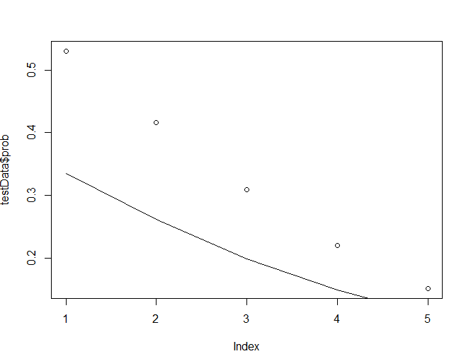
> #其他不变情况下 评级从1到5 婚外情概率从0.53降低至0.15
>
> testData2 <- data.frame(age=seq(17,57,10), rating=mean(Affairs$rating), yearsmarried=mean(Affairs$yearsmarried),
+ religiousness=mean(Affairs$religiousness))
>
> testData2$prob <- predict(fit.some, newdata = testData2, type="response")
>
> #对比图 评级影响更大 更剧烈
> plot(testData$prob)
> lines(testData2$prob)
2、logistics的过度离势

1
2
3
4
5
6
7
8
9
10
11
12
13
14
15
16
17
18
19
20
21
22
> #过度离势
> #过度离势,即观测到的响应变量的方差大于期望的二项分布的方差。过度离势会导致奇异的
> #标准误检验和不精确的显著性检验
> #出现过度离势时,仍可使用glm()函数拟合Logistic回归,但此时需要将二项分布改为类二
> #项分布(quasibinomial distribution)。
> #检测过度离势的一种方法是比较二项分布模型的残差偏差与残差自由度,比值大于1很多表示存在过度离势
> #婚外情中 模型中 Residual deviance: 615.36 on 596 degrees of freedom
> #残差615.36 和 残差自由度596 比值为1.03, 不存在过度离势
>
> #也可使用检验法
> #为此,你需要拟合模型两次,第一次使用family =
> # "binomial",第二次使用family = "quasibinomial"。假设第一次glm()返回对象记为fit.1,
> #第二次返回对象记为fit.2,那么:
> fit.1 <- glm(ynAffair ~ age + yearsmarried + religiousness + rating, data=Affairs,family = binomial())
>
> fit.2 <- glm(ynAffair ~ age + yearsmarried + religiousness + rating, data=Affairs,family = quasibinomial())
>
> pchisq(summary(fit.2)$dispersion * fit.1$df.residual, fit.1$df.residual, lower = F)
[1] 0.340122
> #p值(0.34)显然不显著(p > 0.05),这更增强了我们认为不存在过度离势的信心。
>
>

3、logistics的扩展

1
2
3
4
5
6
7
8
9
10
11
12
> #扩展
>
> #稳健Logistic回归 robust包中的glmRob()函数可用来拟合稳健的广义线性模型,包
> #括稳健Logistic回归。当拟合Logistic回归模型数据出现离群点和强影响点时,稳健Logistic
> #回归便可派上用场。
>
> #多项分布回归 若响应变量包含两个以上的无序类别(比如,已婚/寡居/离婚),便可使
> #用mlogit包中的mlogit()函数拟合多项Logistic回归。
>
> #序数Logistic回归 若响应变量是一组有序的类别(比如,信用风险为差/良/好),便可
> #使用rms包中的lrm()函数拟合序数Logistic回归。
>

4、泊松回归

1
2
3
4
5
6
7
8
9
10
11
12
13
14
15
16
17
18
19
20
21
22
23
24
25
26
27
28
29
30
31
32
> #泊松回归
> #当通过一系列连续型和/或类别型预测变量来预测计数型结果变量时,泊松回归是一个非常
> #有用的工具。
>
> data(breslow.dat, package="robust")
>
> names(breslow.dat)
[1] "ID" "Y1" "Y2" "Y3" "Y4" "Base" "Age" "Trt" "Ysum" "sumY" "Age10"
[12] "Base4"
>
> summary(breslow.dat[c(6,7,8,10)])
Base Age Trt sumY
Min. : 6.00 Min. :18.00 placebo :28 Min. : 0.00
1st Qu.: 12.00 1st Qu.:23.00 progabide:31 1st Qu.: 11.50
Median : 22.00 Median :28.00 Median : 16.00
Mean : 31.22 Mean :28.34 Mean : 33.05
3rd Qu.: 41.00 3rd Qu.:32.00 3rd Qu.: 36.00
Max. :151.00 Max. :42.00 Max. :302.00
>
>
> opar <- par(no.readonly = TRUE)
>
> par(mfrow=c(1,2))
> attach(breslow.dat)
The following objects are masked from breslow.dat (pos = 4):
Age, Age10, Base, Base4, ID, sumY, Trt, Y1, Y2, Y3, Y4, Ysum
>
> hist(sumY, breaks = 20, xlab="Serzure Count", main="Distribution of Serzures")
> boxplot(sumY ~ Trt, xlab="Treatment", main="Group Comparisons")
> par(opar)


1
2
3
4
5
6
7
8
9
10
11
12
13
14
15
16
17
18
19
20
21
22
23
24
25
26
27
28
29
30
31
32
33
34
35
36
37
38
39
> # 拟合泊松回归
> fit <- glm(sumY ~ Base + Age +Trt, data = breslow.dat, family = poisson())
> summary(fit)
Call:
glm(formula = sumY ~ Base + Age + Trt, family = poisson(), data = breslow.dat)
Deviance Residuals:
Min 1Q Median 3Q Max
-6.0569 -2.0433 -0.9397 0.7929 11.0061
Coefficients:
Estimate Std. Error z value Pr(>|z|)
(Intercept) 1.9488259 0.1356191 14.370 < 2e-16 ***
Base 0.0226517 0.0005093 44.476 < 2e-16 ***
Age 0.0227401 0.0040240 5.651 1.59e-08 ***
Trtprogabide -0.1527009 0.0478051 -3.194 0.0014 **
---
Signif. codes: 0 ‘***’ 0.001 ‘**’ 0.01 ‘*’ 0.05 ‘.’ 0.1 ‘ ’ 1
(Dispersion parameter for poisson family taken to be 1)
Null deviance: 2122.73 on 58 degrees of freedom
Residual deviance: 559.44 on 55 degrees of freedom
AIC: 850.71
Number of Fisher Scoring iterations: 5
>
> #泊松回归的因变量以条件均值的对数形式ln(λ)来建模,年龄的回归参数为0.0227,表明
> #保持其他预测变量不变,年龄增加一岁,癫痫发病数的对数均值将相应增加0.03。
> #指数化系数用于方便观察
> exp(coef(fit))
(Intercept) Base Age Trtprogabide
7.0204403 1.0229102 1.0230007 0.8583864
> #保持其他变量不变,年龄增加一岁,期望的癫痫发病数将乘以1.023。
> #与Logistic回归中的指数化参数相似,泊松模型中的指数化参数对响应
> #变量的影响都是成倍增加的,而不是线性相加。
>

5、泊松回归的过度离势

1
2
3
4
5
6
7
8
9
10
11
12
13
14
15
16
17
18
19
20
21
22
23
24
25
26
27
28
29
30
31
32
33
34
35
36
37
38
39
40
41
42
43
44
45
46
47
48
> #泊松分布的过度离势
> #泊松分布的方差和均值相等。当响应变量观测的方差比依据泊松分布预测的方差大时,泊松
> #回归可能发生过度离势。
> #与Logistic回归类似,此处如果残差偏差与残差自由度的比例远远大于1,那么表明存在过度
> #离势。559.44/55 >>1
>
> #qcc包的一个方法可用于检测泊松模型的过度离势
> library(qcc)
> qcc.overdispersion.test(breslow.dat$sumY, type="poisson")
Overdispersion test Obs.Var/Theor.Var Statistic p-value
poisson data 62.87013 3646.468 0
>
> #显著性检验的p值果然小于0.05,进一步表明确实存在过度离势
>
> #此时仍可使用glm进行拟合
> fit.od <- glm(sumY ~ Base + Age +Trt, data = breslow.dat, family = quasipoisson())
> summary(fit.od)
Call:
glm(formula = sumY ~ Base + Age + Trt, family = quasipoisson(),
data = breslow.dat)
Deviance Residuals:
Min 1Q Median 3Q Max
-6.0569 -2.0433 -0.9397 0.7929 11.0061
Coefficients:
Estimate Std. Error t value Pr(>|t|)
(Intercept) 1.948826 0.465091 4.190 0.000102 ***
Base 0.022652 0.001747 12.969 < 2e-16 ***
Age 0.022740 0.013800 1.648 0.105085
Trtprogabide -0.152701 0.163943 -0.931 0.355702
---
Signif. codes: 0 ‘***’ 0.001 ‘**’ 0.01 ‘*’ 0.05 ‘.’ 0.1 ‘ ’ 1
(Dispersion parameter for quasipoisson family taken to be 11.76075)
Null deviance: 2122.73 on 58 degrees of freedom
Residual deviance: 559.44 on 55 degrees of freedom
AIC: NA
Number of Fisher Scoring iterations: 5
> #注意,使用类泊松(quasi-Poisson)方法所得的参数估计与泊松方法相同,但标准误变大
> #了许多。此处,标准误越大将会导致Trt(和Age)的p值越大于0.05。当考虑过度离势,并控
> #制基础癫痫数和年龄时,并没有充足的证据表明药物治疗相对于使用安慰剂能显著降低癫痫发
> #病次数
文章目录
  1. 广义线性模型
    1. 1、广义线性模型和glm函数、logistics回归
    2. 2、logistics的过度离势
    3. 3、logistics的扩展
    4. 4、泊松回归
    5. 5、泊松回归的过度离势