高级图形进阶
1、lattice
1 2 3 4 5 6 7
| library(lattice) histogram(~height|voice.part, data = singer, main="合唱团身高和声部的分布", xlab="身高(英尺)")
|

1 2 3 4 5 6 7 8 9
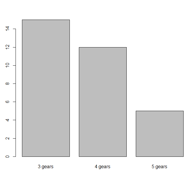
| library(lattice) attach(mtcars) gearPlot <- factor(mtcars$gear, levels = c(3, 4, 5), labels = c("3 gears", "4 gears", "5 gears")) plot(gearPlot)
|
1 2 3
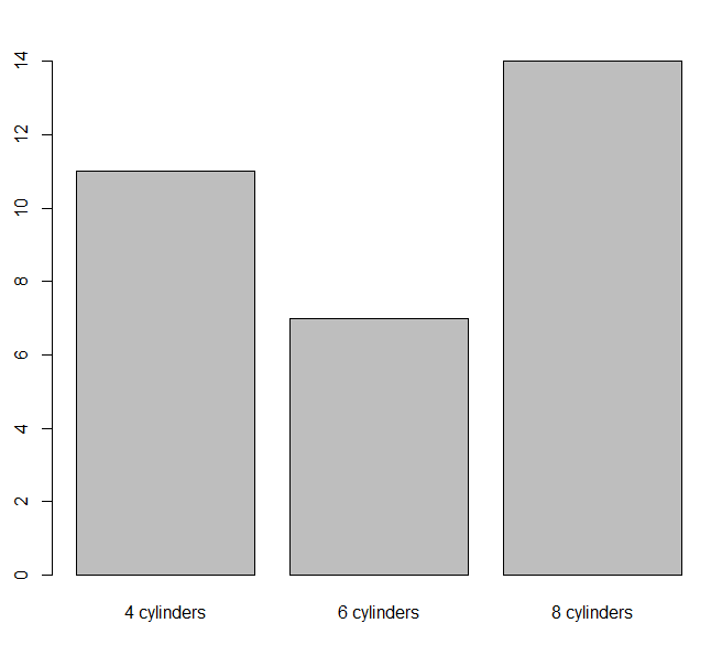
| cylPlot <- factor(mtcars$cyl, levels = c(4, 6, 8), labels = c("4 cylinders", "6 cylinders", "8 cylinders")) plot(cylPlot)
|
1 2
| densityplot(~mpg, main = "核密度图", xlab = "每加仑的英里数")
|

1 2 3
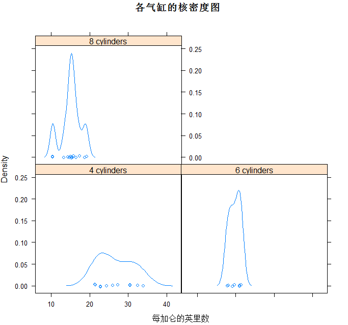
| densityplot(~mpg | cyl, main = "各气缸的核密度图", xlab = "每加仑的英里数")
|
1 2 3
| bwplot(cyl ~ mpg | gear, main = "气缸和档数的箱线图", xlab = "英里每加仑", ylab = "气缸数")
|

1 2 3
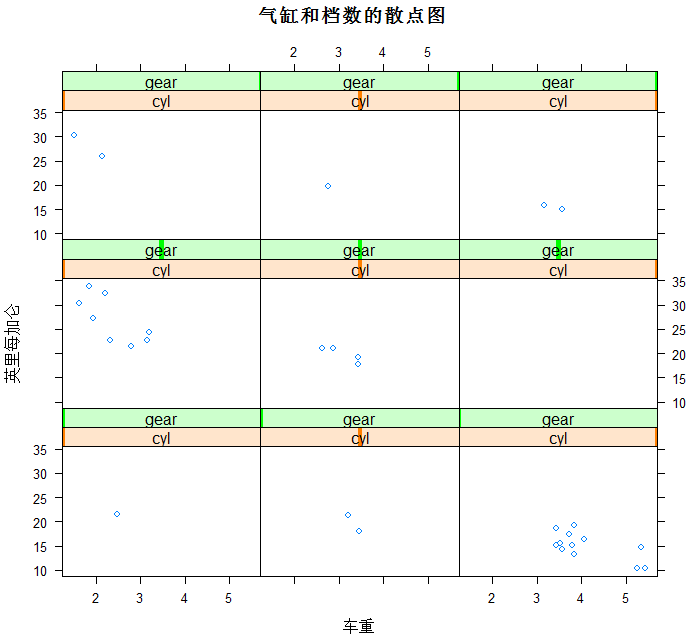
| xyplot(mpg ~ wt | cyl * gear, main = "气缸和档数的散点图", xlab = "车重", ylab = "英里每加仑")
|
1 2 3
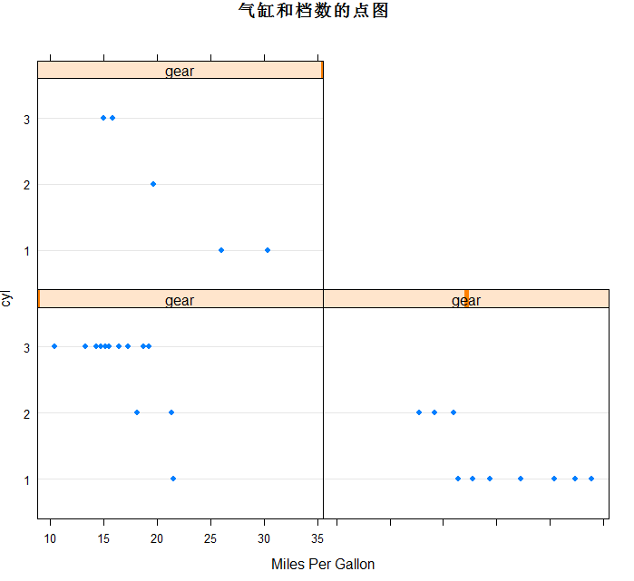
| dotplot(cyl ~ mpg | gear, main = "气缸和档数的点图", xlab = "Miles Per Gallon")
|
1 2
| cloud(mpg ~ wt * qsec | cyl, main = "各气缸的3D散点图")
|

1 2 3 4 5
| splom(mtcars[c(1, 3, 4, 5, 6)], main = "散点矩阵图") detach(mtcars)
|

1 2 3 4
| myg <-densityplot(~height | voice.part, data=singer) update(myg, col="red", pch=16, cex=.8, lwd=2)
|

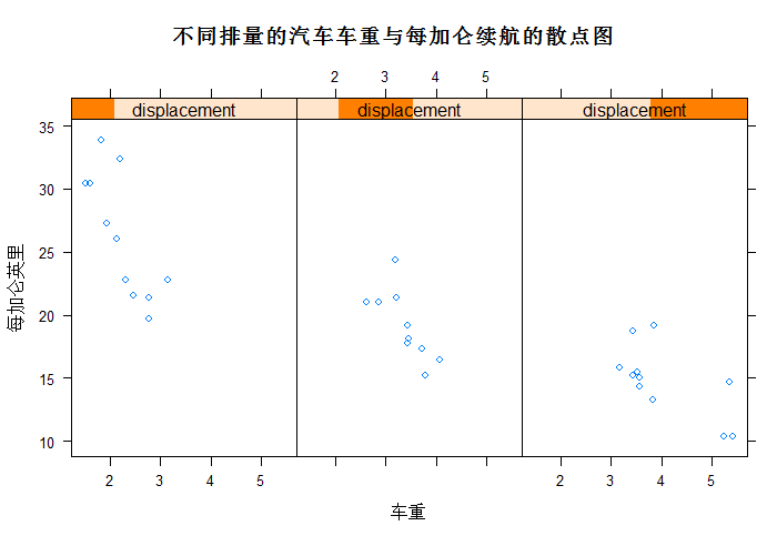
1、条件变量
1 2 3 4 5 6 7
| displacement <- equal.count(mtcars$disp, number = 3, overlap = 0) xyplot(mpg ~ wt | displacement, data = mtcars, main = "不同排量的汽车车重与每加仑续航的散点图", xlab = "车重", ylab = "每加仑英里", layout = c(3, 1), aspect = 1.5)
|
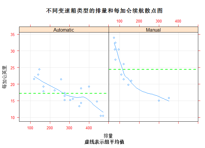
2、面板函数
1 2 3 4 5 6 7 8 9 10 11 12 13 14 15
| displacement <- equal.count(mtcars$disp, number = 3, overlap = 0) mypanel <- function(x, y) { panel.xyplot(x, y, pch = 19) panel.rug(x, y) panel.grid(h = -1, v = -1) panel.lmline(x, y, col = "red", lwd = 1, lty = 2) } xyplot(mpg ~ wt | displacement, data = mtcars, layout = c(3, 1), aspect = 1.5, main = "不同排量的汽车车重与每加仑续航的散点图(自定义面板函数)", xlab = "车重", ylab = "每加仑英里", panel = mypanel)
|

1 2 3 4 5 6 7 8 9 10 11 12 13 14 15 16 17 18 19
| library(lattice) mtcars$transmission <- factor(mtcars$am, levels = c(0, 1), labels = c("Automatic", "Manual")) panel.smoother <- function(x, y) { panel.grid(h = -1, v = -1) panel.xyplot(x, y) panel.loess(x, y) panel.abline(h = mean(y), lwd = 2, lty = 2, col = "green") } xyplot(mpg ~ disp | transmission, data = mtcars, scales = list(cex = 0.8, col = "red"), panel = panel.smoother, xlab = "排量", ylab = "每加仑英里", main = "不同变速箱类型的排量和每加仑续航散点图", sub = "虚线表示组平均值", aspect = 1)
|
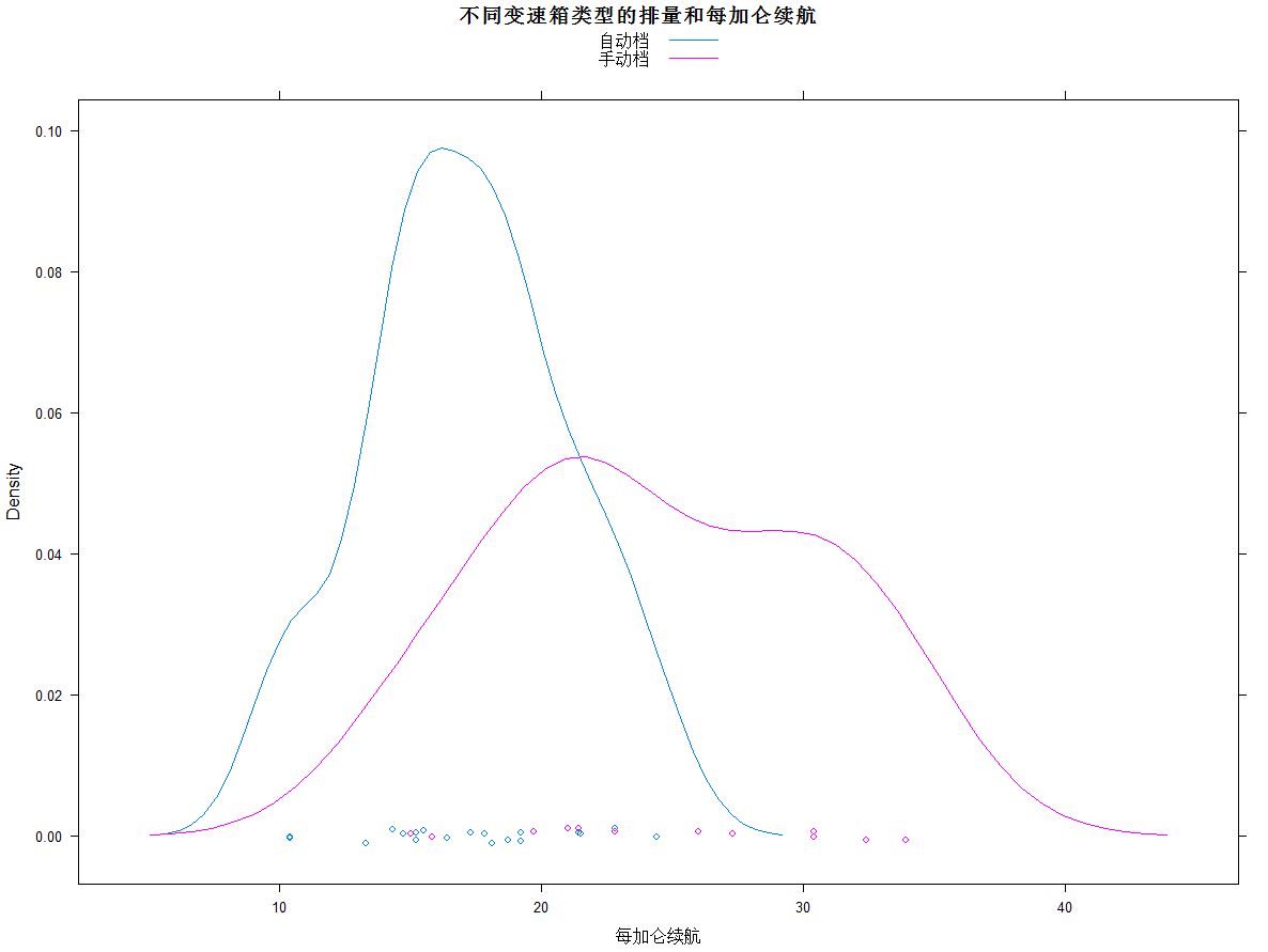
3、分组变量,多个面板的数据合一
1 2 3 4 5 6 7 8
| library(lattice) mtcars$transmission <- factor(mtcars$am, levels = c(0, 1), labels = c("自动档", "手动档")) densityplot(~mpg, data = mtcars, group = transmission, main = "不同变速箱类型的排量和每加仑续航", xlab = "每加仑续航", auto.key = TRUE)
|
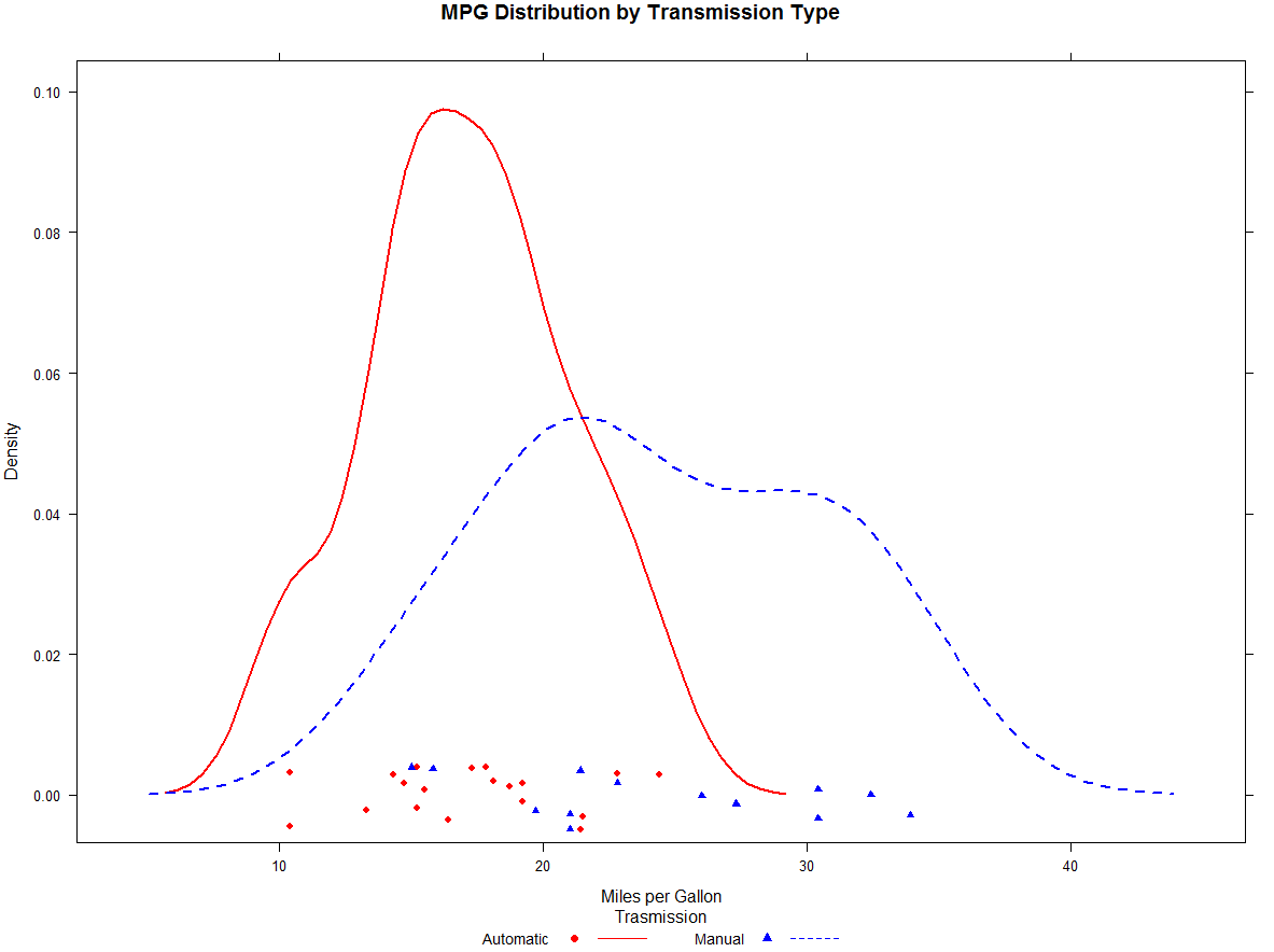
1 2 3 4 5 6 7 8 9 10 11 12 13 14 15 16 17 18 19 20 21 22 23 24 25
| library(lattice) mtcars$transmission <- factor(mtcars$am, levels = c(0, 1), labels = c("Automatic", "Manual")) colors = c("red", "blue") lines = c(1, 2) points = c(16, 17) key.trans <- list(title = "传动方式", space = "bottom", columns = 2, text = list(levels(mtcars$transmission)), points = list(pch = points, col = colors), lines = list(col = colors, lty = lines), cex.title = 1, cex = 0.9) densityplot(~mpg, data = mtcars, group = transmission, main = "不同变速箱类型的排量和每加仑续航", xlab = "每加仑续航", pch = points, lty = lines, col = colors, lwd = 2, jitter = 0.005, key = key.trans)
|
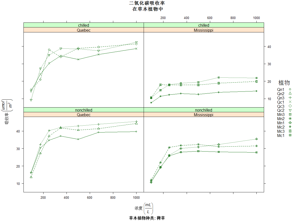
1 2 3 4 5 6 7 8 9 10 11 12 13 14 15 16 17 18 19 20 21 22
| library(lattice) colors <- "darkgreen" symbols <- c(1:12) linetype <- c(1:3) key.species <- list(title = "植物", space = "right", text = list(levels(CO2$Plant)), points = list(pch = symbols, col = colors)) xyplot(uptake ~ conc | Type * Treatment, data = CO2, group = Plant, type = "o", pch = symbols, col = colors, lty = linetype, main = "二氧化碳吸收率\n 在草本植物中", ylab = expression(paste("吸收率 ", bgroup("(", italic(frac("umol", "m"^2)), ")"))), xlab = expression(paste("浓度 ", bgroup("(", italic(frac(mL, L)), ")"))), sub = "草本植物种类: 稗草", key = key.species)
|
4、lattice的图形参数
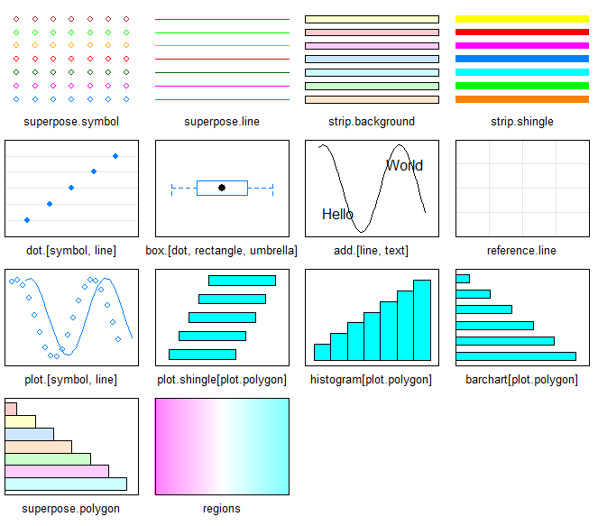
1 2 3 4 5 6 7 8 9 10
| show.settings() mysettings <- trellis.par.get() mysettings$superpose.symbol mysettings$superpose.symbol$pch <- c(1:10) trellis.par.set(mysettings) show.settings()
|
5、图形摆放
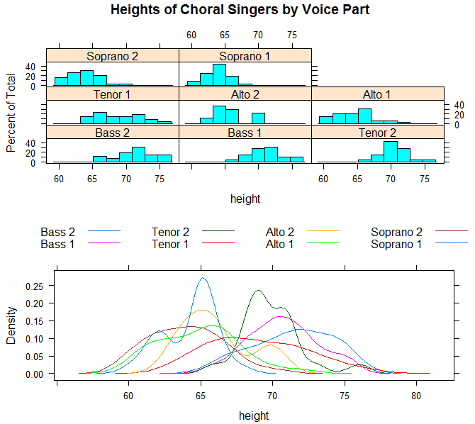
1 2 3 4 5 6 7 8 9
| library(lattice) graph1 <- histogram(~height | voice.part, data = singer, main = "Heights of Choral Singers by Voice Part") graph2 <- densityplot(~height, data = singer, group = voice.part, plot.points = FALSE, auto.key = list(columns = 4)) plot(graph1, split = c(1, 1, 1, 2)) plot(graph2, split = c(1, 2, 1, 2), newpage = FALSE)
|
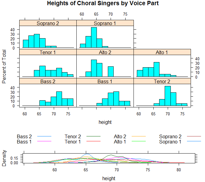
1 2 3 4 5 6 7 8
| library(lattice) graph1 <- histogram(~height | voice.part, data = singer, main = "Heights of Choral Singers by Voice Part") graph2 <- densityplot(~height, data = singer, group = voice.part, plot.points = FALSE, auto.key = list(columns = 4)) plot(graph1, position = c(0, 0.3, 1, 1)) plot(graph2, position = c(0, 0, 1, 0.3), newpage = FALSE)
|
2、ggplot2包
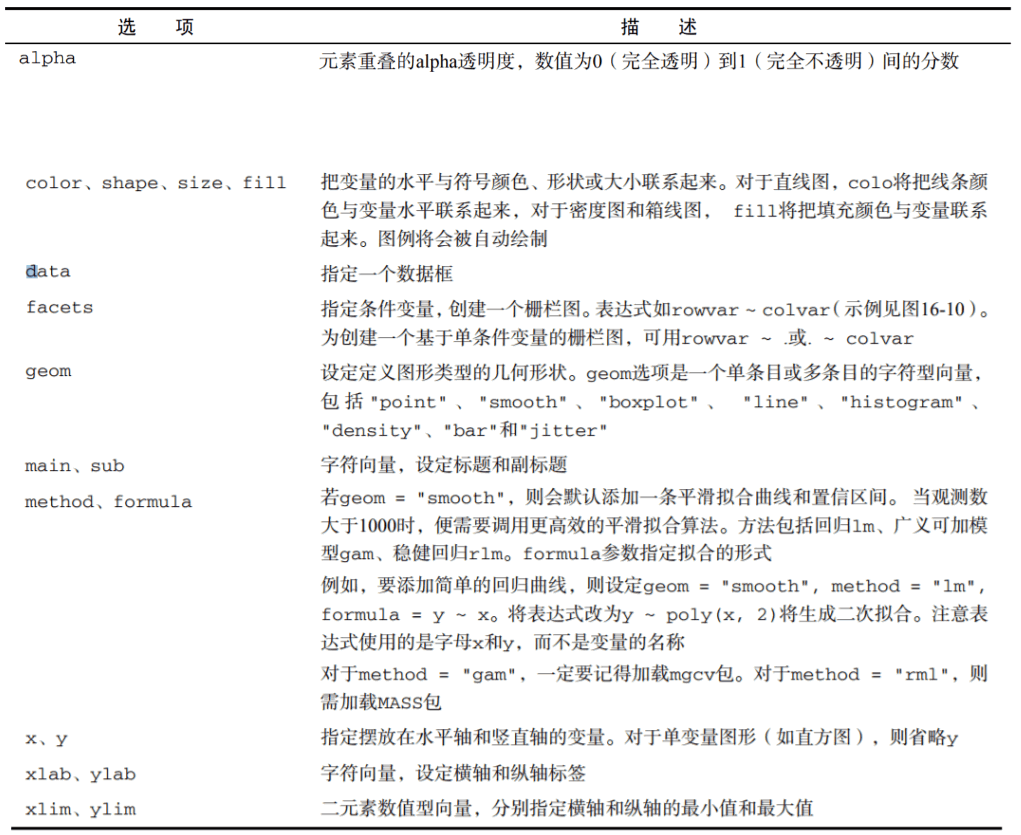
1 2 3 4 5 6 7 8
| library(ggplot2) mtcars$cylinder <- as.factor(mtcars$cyl) qplot(cylinder, mpg, data=mtcars, geom=c("boxplot", "jitter"), fill=cylinder, main="叠加数据点的箱线图", xlab= "气缸数", ylab="每加仑续航")
|

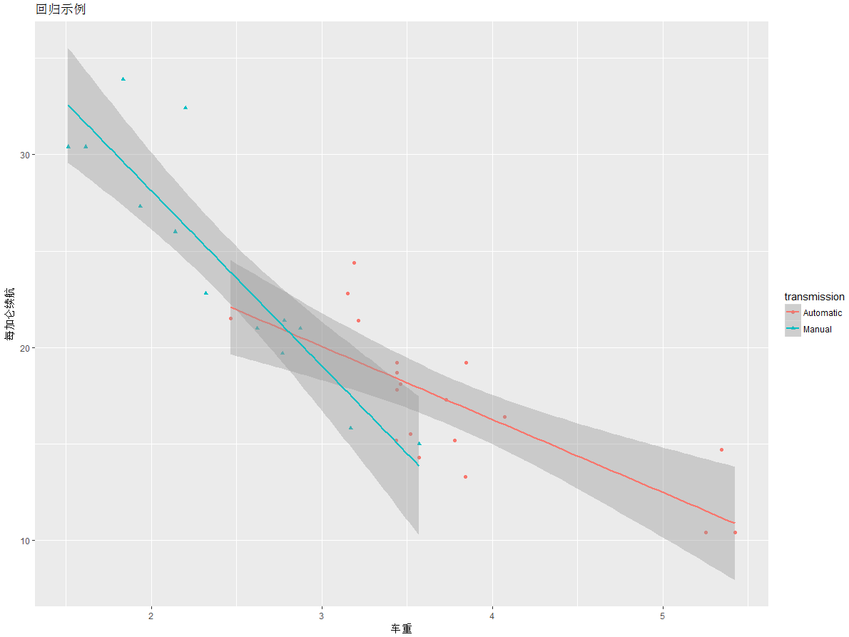
1 2 3 4 5 6 7 8 9 10
| library(ggplot2) transmission <- factor(mtcars$am, levels = c(0, 1), labels = c("自动", "手动")) qplot(wt, mpg, data = mtcars, color = transmission, shape = transmission, geom = c("point", "smooth"), method = "lm", formula = y ~ x, xlab = "车重", ylab = "每加仑续航", main = "回归示例")
|
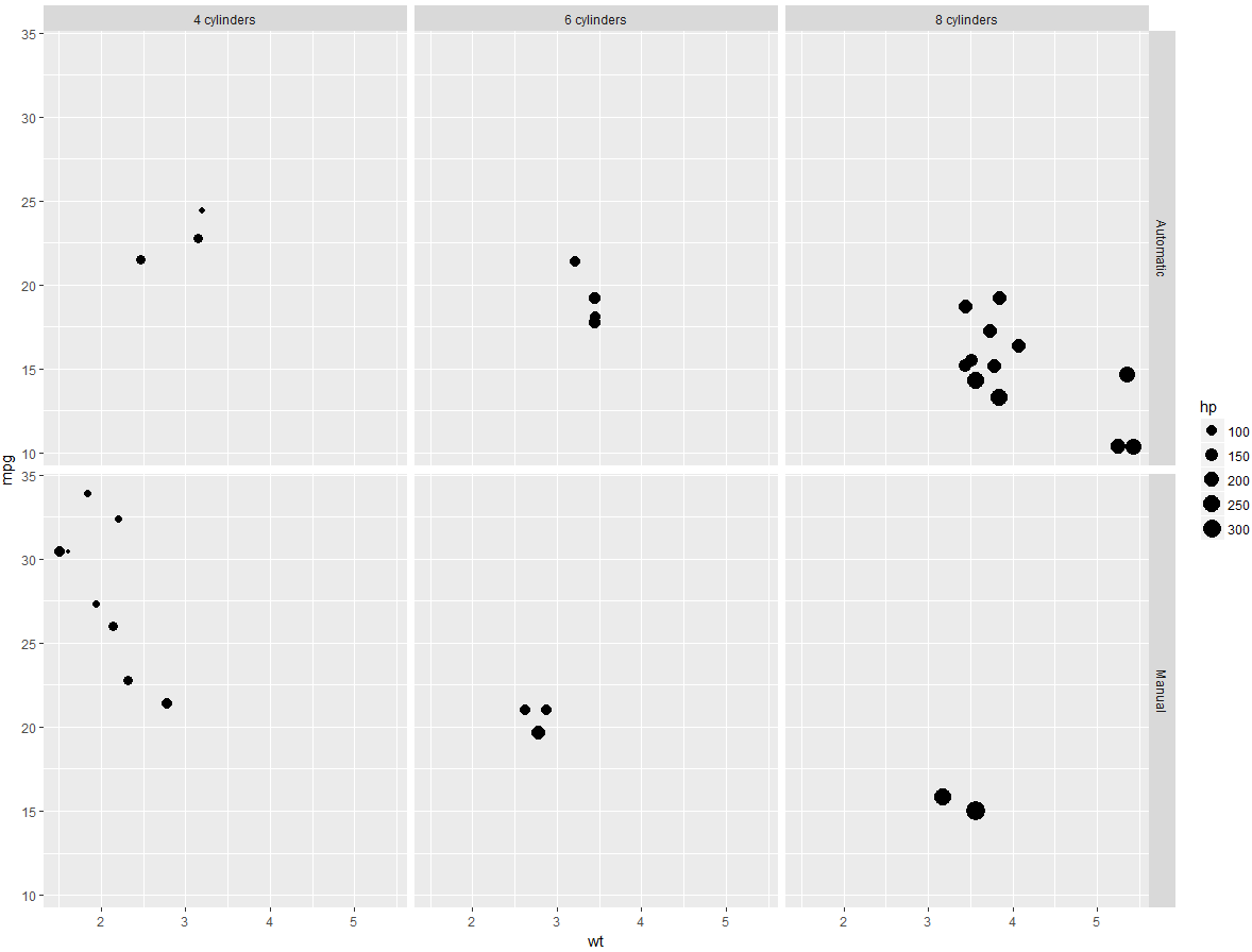
1 2 3 4 5 6 7
| library(ggplot2) mtcars$cyl <- factor(mtcars$cyl, levels = c(4, 6, 8), labels = c("4 cylinders", "6 cylinders", "8 cylinders")) mtcars$am <- factor(mtcars$am, levels = c(0, 1), labels = c("Automatic", "Manual")) qplot(wt, mpg, data = mtcars, facets = am ~ cyl, size = hp)
|
1 2 3 4 5 6
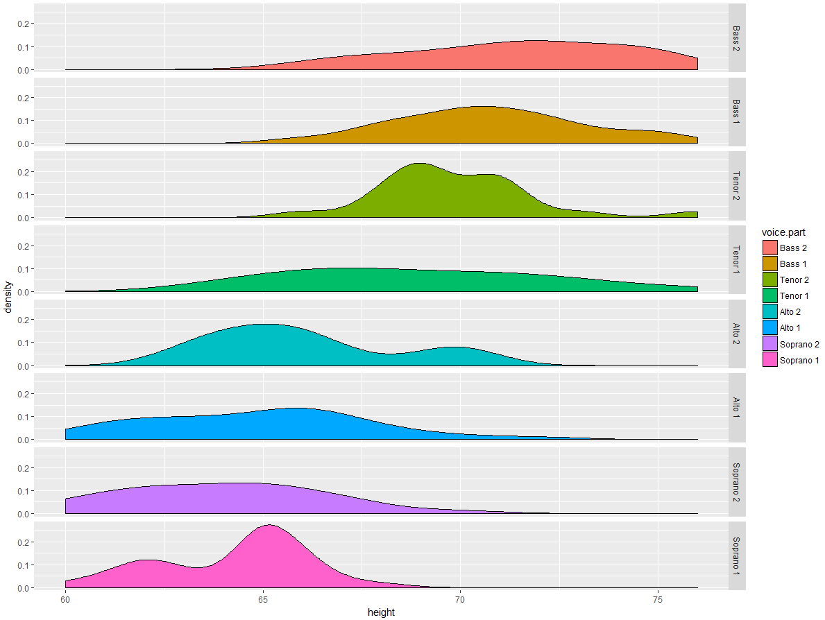
| library(ggplot2) data(singer, package = "lattice") qplot(height, data = singer, geom = c("density"), facets = voice.part ~ ., fill = voice.part)
|